Mastering Pareto Charts In Excel: A Complete Information

Mastering Pareto Charts in Excel: A Complete Information

Associated Articles: Mastering Pareto Charts in Excel: A Complete Information

Introduction

With enthusiasm, let’s navigate via the intriguing subject associated to Mastering Pareto Charts in Excel: A Complete Information. Let’s weave fascinating data and provide recent views to the readers.

Mastering Pareto Charts in Excel: A Complete Information

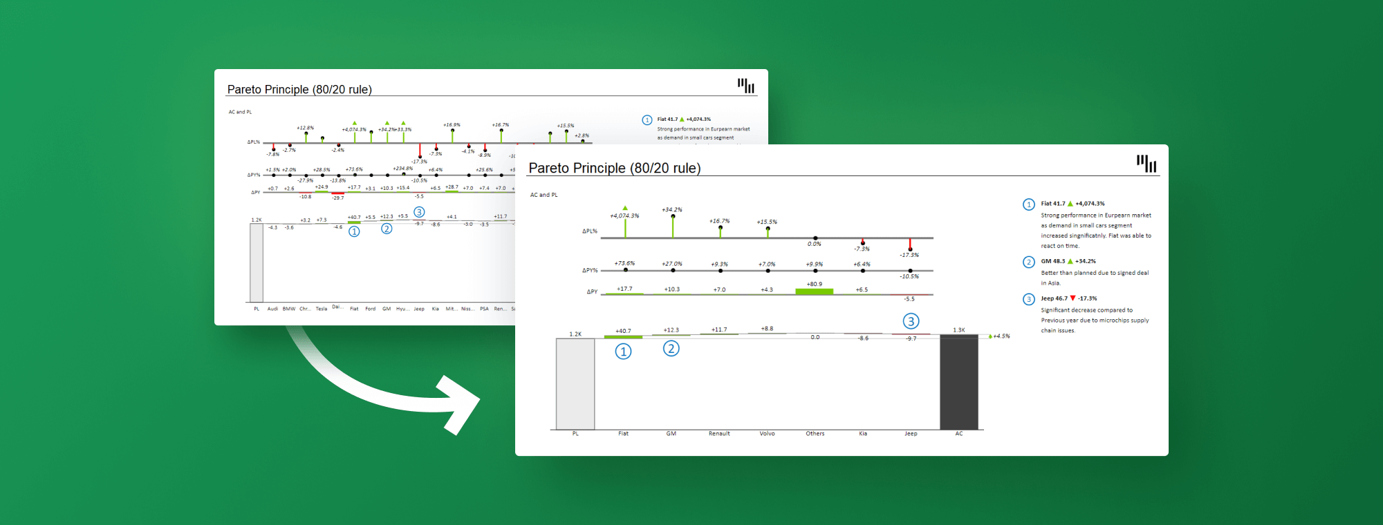
The Pareto precept, famously often known as the "80/20 rule," means that roughly 80% of results come from 20% of causes. Visualizing this precept successfully is essential for figuring out key areas needing consideration, whether or not in enterprise, manufacturing, or private initiatives. The Pareto chart, a mixture bar and line graph, excels at this process. This text supplies a complete information to creating and deciphering Pareto charts in Microsoft Excel, masking numerous eventualities and superior methods.

Understanding the Pareto Chart:

A Pareto chart concurrently shows each the frequency of various classes and their cumulative frequency. The classes are usually organized in descending order of frequency, permitting for rapid identification of the "very important few" contributing to nearly all of the issue or final result. The bar chart represents the person class frequencies, whereas the road graph reveals the cumulative proportion. This twin illustration powerfully highlights the disproportionate influence of a small variety of classes.

Knowledge Preparation: The Basis of Efficient Pareto Charts:

Earlier than diving into Excel, meticulous knowledge preparation is crucial. This entails:

1. Knowledge Assortment: Collect correct and related knowledge representing the classes and their corresponding frequencies. This may very well be the variety of defects by kind, buyer complaints by supply, gross sales by product, or another related metric. Guarantee your knowledge is clear and constant.

2. Knowledge Group: Manage your knowledge right into a structured format, usually a desk with two columns: one for the class (e.g., defect kind) and one for its frequency (e.g., variety of defects).

3. Knowledge Sorting: Kind the classes in descending order primarily based on their frequency. That is essential for the visible influence of the Pareto chart. Excel’s sorting performance makes this simple.

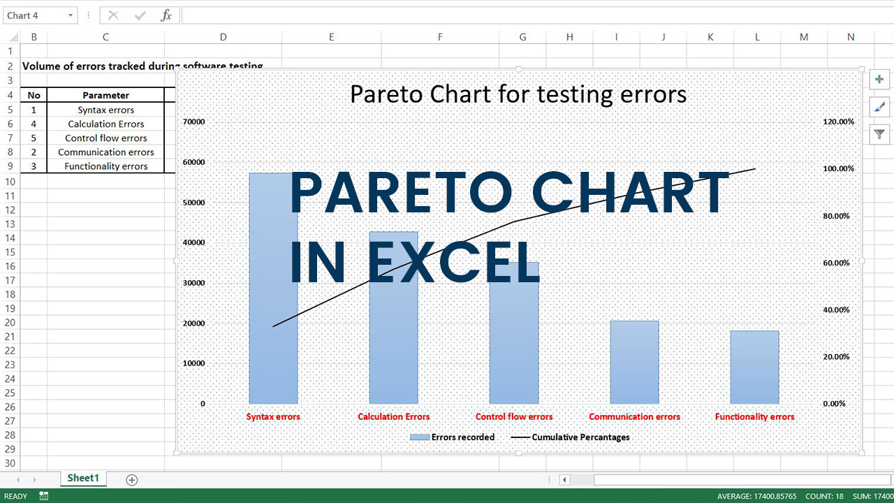
Making a Pareto Chart in Excel: A Step-by-Step Information:

Excel gives a number of methods to create a Pareto chart. We’ll discover two frequent approaches: utilizing the built-in chart options and leveraging PivotTables for extra dynamic evaluation.

Methodology 1: Utilizing Excel’s Constructed-in Charting Options:

This technique is appropriate for smaller datasets and easier eventualities.

1. Put together your knowledge: Manage your knowledge as described above, with classes in descending order of frequency.

2. Insert a chart: Choose your knowledge (each classes and frequencies). Go to the "Insert" tab and select "Insert Column or Bar Chart." Choose a clustered column chart.

3. Add the cumulative proportion line: That is the important thing to reworking a easy bar chart right into a Pareto chart. You will have to calculate the cumulative proportion. In a brand new column subsequent to your frequency knowledge, calculate the cumulative proportion utilizing the SUM operate and dividing by the whole frequency. For instance, in case your frequency column is B, the cumulative proportion system in cell C2 could be =SUM($B$2:B2)/SUM($B$2:$B$10) (assuming 10 knowledge factors). Drag this system down.

4. Add the road chart: Choose your cumulative proportion knowledge. Proper-click and select "Choose Knowledge." Click on "Add" and title the collection (e.g., "Cumulative Share"). Choose the vary containing your cumulative percentages. Click on "OK" twice. You now have a mixture chart.

5. Format the chart: Customise the chart’s look (titles, labels, colours, and so forth.) for readability {and professional} enchantment. Take into account including knowledge labels to each the bars and the road for enhanced readability.

Methodology 2: Leveraging PivotTables for Dynamic Evaluation:

This strategy is extremely really useful for bigger datasets and eventualities requiring versatile evaluation.

1. Create a PivotTable: Choose your knowledge and go to the "Insert" tab. Select "PivotTable." Choose the place you need to place the PivotTable.

2. Configure the PivotTable: Drag the class area to the "Rows" space and the frequency area to the "Values" space. Excel robotically sums the frequencies.

3. Add the cumulative proportion: Proper-click on any frequency worth within the PivotTable. Choose "Present Values As" -> "% of Grand Whole." This may add a brand new column with cumulative percentages.

4. Create a Pareto Chart from the PivotTable: Choose the PivotTable. Go to the "Insert" tab and select a clustered column chart. Excel will robotically create a chart primarily based in your PivotTable knowledge, together with the cumulative percentages.

5. Format the chart: Customise the chart’s look as wanted.

Decoding the Pareto Chart:

The Pareto chart’s energy lies in its visible illustration of the 80/20 rule. By shortly figuring out the few classes contributing to nearly all of the issue or final result, you may prioritize your efforts.

• The "Very important Few": The leftmost bars symbolize probably the most important contributors. Focus your assets and a spotlight on addressing these classes first.

• The "Trivial Many": The rightmost bars symbolize classes with smaller contributions. Whereas necessary, addressing these is perhaps much less impactful than specializing in the "very important few."

• Cumulative Share Line: The road graph showcases the cumulative influence of addressing classes sequentially. It helps visualize the purpose at which addressing extra classes yields diminishing returns.

Superior Methods and Concerns:

• Weighted Pareto Charts: For conditions the place classes have totally different weights or significance, you may create weighted Pareto charts by incorporating weights into your calculations.

• Pareto Charts with A number of Variables: You’ll be able to create extra advanced Pareto charts to investigate a number of variables concurrently, offering a richer understanding of the underlying relationships.

• Dynamic Pareto Charts: Utilizing PivotTables lets you dynamically replace the chart primarily based on totally different knowledge filters or alternatives.

Conclusion:

Pareto charts are highly effective instruments for visualizing the 80/20 rule and prioritizing efforts. Excel supplies versatile instruments to create and interpret these charts successfully. By mastering the methods outlined on this article, you may leverage the Pareto precept to enhance decision-making and obtain higher effectivity in numerous facets of your work and life. Keep in mind that the important thing to a profitable Pareto chart lies in correct knowledge preparation and considerate interpretation of the ensuing visualization. By fastidiously choosing your knowledge and customizing your chart, you may unlock beneficial insights and optimize your strategy to problem-solving and useful resource allocation.

Closure

Thus, we hope this text has offered beneficial insights into Mastering Pareto Charts in Excel: A Complete Information. We hope you discover this text informative and useful. See you in our subsequent article!