Reworking Chart 1 Into Chart 2: A Complete Information To Excel Chart Manipulation

Reworking Chart 1 into Chart 2: A Complete Information to Excel Chart Manipulation

Associated Articles: Reworking Chart 1 into Chart 2: A Complete Information to Excel Chart Manipulation

Introduction

With enthusiasm, let’s navigate via the intriguing subject associated to Reworking Chart 1 into Chart 2: A Complete Information to Excel Chart Manipulation. Let’s weave fascinating data and provide recent views to the readers.

Reworking Chart 1 into Chart 2: A Complete Information to Excel Chart Manipulation

Excel’s charting capabilities are extremely versatile, permitting customers to remodel uncooked knowledge into visually compelling and informative representations. Typically, nevertheless, the preliminary chart generated by Excel does not completely align with the specified visualization. This text delves into the method of modifying an current Excel chart (Chart 1) to resemble a goal chart (Chart 2), offering an in depth walkthrough encompassing numerous methods and concerns. We’ll discover situations requiring changes to chart sort, knowledge illustration, styling, and total structure, aiming to equip readers with the talents to attain subtle chart transformations.

Understanding the Transformation Course of:

Earlier than embarking on the transformation, an intensive understanding of each Chart 1 and Chart 2 is essential. This contains:

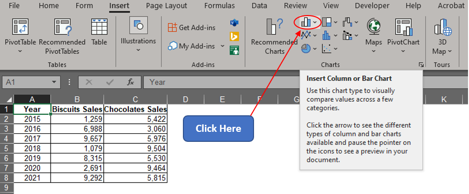
• Chart Kind: Are each charts of the identical sort (e.g., bar chart, line chart, pie chart)? If not, changing between chart sorts is step one. This usually includes deciding on the chart, navigating to the "Change Chart Kind" choice, and deciding on the specified sort from the obtainable choices. Concerns embody the suitability of the brand new chart sort for the info being represented.

• Information Illustration: How is the info introduced in every chart? Chart 1 may use clustered columns, whereas Chart 2 may require stacked columns or a 100% stacked column chart. Equally, line charts may should be adjusted to indicate totally different knowledge collection, smoothed strains, or markers. This step requires cautious evaluation of the info and the way it must be reorganized throughout the chart. Typically, this includes manipulating the underlying knowledge within the spreadsheet itself earlier than making modifications to the chart.

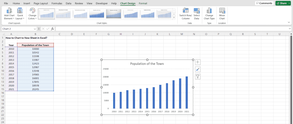
• Axes and Labels: The x-axis and y-axis labels, titles, and items of measurement should be meticulously examined. Chart 1 may need generic labels, whereas Chart 2 may require particular, descriptive labels. Adjusting these parts includes deciding on the axis, accessing the formatting choices, and modifying the textual content, quantity format, and different properties.

• Chart Parts: This contains parts like legends, knowledge labels, gridlines, titles, and chart borders. Chart 1 may need a legend positioned in a suboptimal location, whereas Chart 2 may require a legend with personalized formatting and even the elimination of the legend altogether. Information labels, if current, may should be repositioned, formatted in a different way (e.g., exhibiting percentages as an alternative of values), or added altogether. Gridlines can improve readability or litter the chart, relying on the context, and their inclusion or exclusion ought to be fastidiously thought-about.

• Colours and Types: The colour palette, font kinds, and total aesthetic of Chart 1 may differ considerably from Chart 2. Excel provides a variety of customization choices for colours, fonts, and fill patterns. Consistency in styling is essential for making a visually interesting {and professional} chart. Think about using Excel’s built-in themes or making a customized theme for a unified look.

Step-by-Step Transformation Strategies:

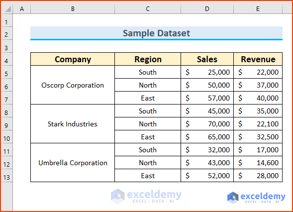
Let’s assume Chart 1 is a straightforward column chart exhibiting gross sales knowledge for 3 merchandise over 4 quarters, and Chart 2 is a extra subtle chart with stacked columns, knowledge labels exhibiting percentages, a customized title, and a selected colour scheme.

1. Information Preparation: Start by making certain the info in your spreadsheet is organized appropriately for the specified chart sort in Chart 2. This may contain pivoting tables, including calculated fields, or just rearranging columns and rows.

2. Chart Kind Conversion: If Chart 1 isn’t already a stacked column chart, choose it and navigate to "Change Chart Kind." Select the "Stacked Column" choice.

3. Information Sequence Administration: Guarantee the proper knowledge collection are stacked appropriately. Excel may mechanically assign collection, however guide adjustment is perhaps essential to attain the specified stacking order.

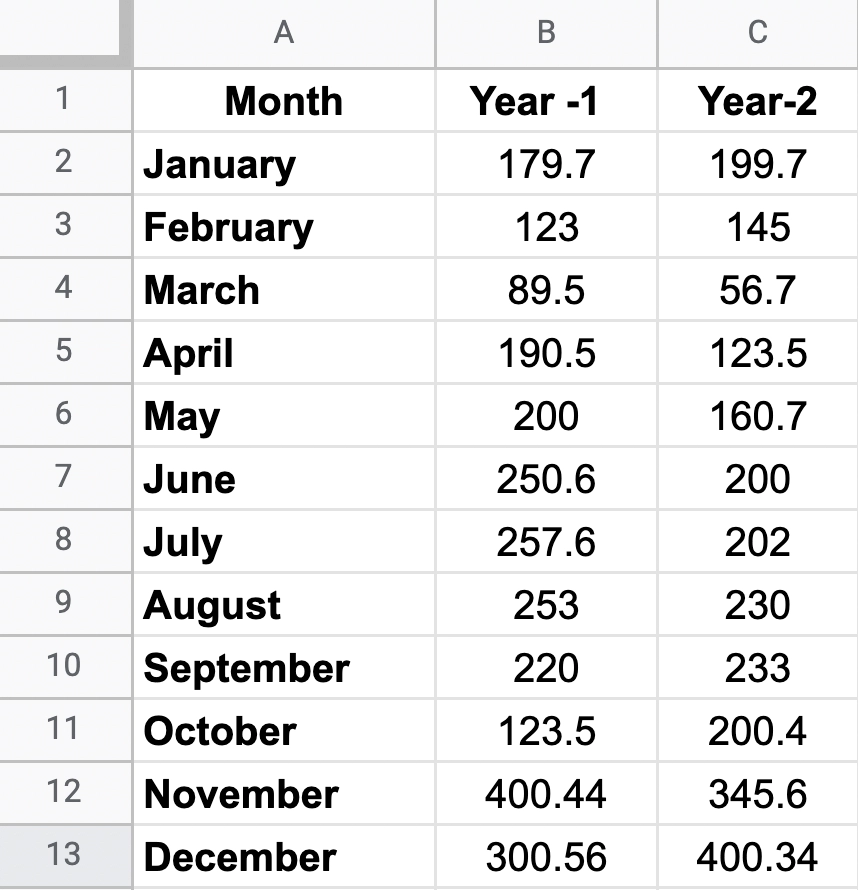
4. Axis and Labels: Edit the axis labels to mirror the particular time intervals (quarters) and product names. Customise the axis titles to be clear and descriptive. Think about including items (e.g., "Gross sales in Hundreds").

5. Information Labels: Add knowledge labels to every column phase. Format these labels to show percentages as an alternative of uncooked values. This requires deciding on the info labels, accessing the formatting choices, and selecting the proportion format. Place the labels strategically for optimum readability.

6. **Chart

Closure

Thus, we hope this text has supplied invaluable insights into Reworking Chart 1 into Chart 2: A Complete Information to Excel Chart Manipulation. We hope you discover this text informative and helpful. See you in our subsequent article!